Contents
Project overview#
![]()

![]()
![]()
High-fidelity simulator for synthetic IFU (Integral Field Unit) spectral cubes.#
GalCubeCraft provides a compact, well-documented pipeline to build 3D spectral cubes that mimic observations of disk galaxies. It combines simple analytic galaxy models (Sérsic light profiles + exponential vertical structure), simple rotation-curve kinematics, viewing-angle projections and instrument effects (beam convolution, channel binning) to produce a physically motivated basis and test data for algorithm development, denoising, and visualization.
This README explains the science and mathematics behind the generator, how to install the package, and several practical examples for quick experimentation.
Table of contents#
What GalCubeCraft does
Scientific background & equations
Installation (PyPI + source)
Quick start examples
API reference (minimal)
Reproducibility, limitations, and troubleshooting
Credits & citation
What GalCubeCraft does#
GalCubeCraft synthesizes spectral datacubes with dimensions \((n_s, n_y, n_x)\). Each cube contains one or more galaxy components. For each galaxy component the generator:
Builds a 3D flux density field using a Sérsic profile in the disk plane combined with an exponential vertical profile.
Computes an analytic circular velocity field from a compact rotation-curve model and assigns tangential velocities to voxels.
Rotates the 3D flux and velocity fields to a chosen viewing geometry.
Projects emission into line-of-sight velocity bins to produce a spectral cube.
Optionally convolves each 2D channel with a telescope beam and saves cubes to
data/raw_data/<nz>x<ny>x<nx>/cube_*.npy.
The package is intentionally clear and inspectable (readable loops, compact functions), making it suitable for method development and teaching.
Scientific background & equations#
This section summarises the main mathematical building blocks implemented in the code: the Sérsic flux distribution, vertical exponential profile, and the analytical rotation curve used to assign tangential velocities.
Sérsic radial profile (disk plane)#
The radial surface brightness (Sérsic) profile is given by
where
\(S_e\) is the flux density at the effective radius \(R_e\),
\(n\) is the Sérsic index that controls the concentration,
\(b_n\) is a constant that depends on \(n\) (approximated by a series expansion).
The package uses the standard series expansion for \(b_n\):
Vertical exponential profile#
Galaxies are modeled with an exponential vertical fall-off:
Combining radial and vertical profiles gives the 3D flux density used in the generator:
with \(r = \sqrt{x^2 + y^2}\) in the disk plane.
Analytical rotation curve#
To assign tangential velocities the implementation uses a compact empirical
approximation (implemented as milky_way_rot_curve_analytical):
where \(v_0\) is a characteristic velocity scale and \(R_0\) is derived from the effective radius and Sérsic index (see code comments for details). This simple form reproduces the gently rising/flat behaviour of typical disk-galaxy rotation curves at the scales of interest for IFU-like synthetic data.
Beam convolution and FWHM to σ relation#
When simulating instrument resolution we convolve 2D channels with an elliptical Gaussian. The conversion between FWHM and Gaussian sigma used is:
This relation is used when creating a Gaussian2DKernel for convolution.
Installation#
pip install GalCubeCraft
Installing from source (developer mode):
git clone https://github.com/arnablahiry/GalCubeCraft.git
cd GalCubeCraft
pip install -e .
Recommended dependencies are listed in requirements.txt. A minimal set used by
the package includes:
numpy
scipy
matplotlib
astropy
torch
If you rely on plotting or dendrograms, also ensure astrodendro is available:
pip install astrodendro
Note: for environments with GPU-accelerated PyTorch, install a matching torch
build according to your CUDA version (see https://pytorch.org).
Quick start examples#
Below are short, runnable examples that demonstrate common workflows. The examples assume a Python session or script; replace package name with the one you published to PyPI if different.
1) Generate one synthetic cube and inspect shapes#
from GalCubeCraft import GalCubeCraft

# Create a generator: one cube, grid 125x125, 40 spectral channels (internally oversampled)
g = GalCubeCraft(n_gals=None, n_cubes=1, resolution='all', grid_size=125, n_spectral_slices=40, seed=42)

# Run the generation pipeline and collect results
results = g.generate_cubes()

# Each element in results is a tuple (spectral_cube, params_dict)

cube, params_dict = results[0]
print('cube shape (nz, ny, nx) =', cube.shape)
print('geenration parameter keys =', list(params_dict.keys()))
Typical output:
cube.shape→ (n_velocity, ny, nx) (e.g. (40, 125, 125))params_dictcontainsaverage_vels,beam_info,pix_spatial_scale, etc.
2) Save and visualise#
GalCubeCraft saves generated cubes to data/raw_data/<nz>x<ny>x<nx>/cube_*.npy by
default. The class also exposes a visualise helper that wraps the plotting
helpers in visualise.py:
g.visualise(results, idx=0, save=False)
This will show moment-0 and moment-1 maps and a velocity spectrum using
matplotlib. Set save=True to write PDF figures in figures/<shape>/.
Use as a coarse dataset for transfer learning#
GalCubeCraft is intentionally fast, controllable, and able to produce large numbers of cubes with varied orientations, resolutions, surface-brightness scalings and noise behaviour. For these reasons it makes a robust coarse dataset to pretrain machine-learning models before fine-tuning on smaller, scientifically complex datasets.
Recommended workflow:
Pretrain on large GalCubeCraft datasets to learn general spectro-spatial features (correlated spectral lines, beam-smearing patterns, moment-map structure). Vary resolution, S/N, Sérsic index and component multiplicity to expose the model to a broad prior.
Fine-tune on a much smaller but higher-fidelity dataset that explicitly includes the morphological complexities your downstream task requires — for example gravitational lensing distortions, diffuse low-surface-brightness emission, bridges and tidal tails from interacting systems, multi-component kinematics, or instrument-specific artifacts.
Why this helps:
Reduces overfitting to small labelled sets by learning lower-level features on the synthetic data and adapting higher-level representations to the target domain during fine-tuning.
Speeds training and improves sample efficiency when real or high-fidelity labels are scarce or expensive to create.
Practical tips:
Freeze early convolutional layers (or set a low learning rate) during initial fine-tuning to preserve general features learned from GalCubeCraft.
Use domain adaptation techniques (data augmentation, style transfer, or adversarial domain adaptation) to close the gap between synthetic and real observations.
When you need morphological realism (lensing, bridges, tails, diffuse emission), either augment GalCubeCraft procedurally (apply lensing transforms, add low-surface-brightness components, overlay tidal bridges) or fine-tune on simulation/observation datasets that include such complexity.
Example tasks that benefit from this workflow: denoising, deconvolution, source detection/segmentation, kinematic parameter regression, and anomaly detection in spectral cubes.
Minimal API reference#
GalCubeCraft(n_gals=None, n_cubes=1, resolution='all', offset_gals=5, beam_info=[4,4,0], grid_size=125, n_spectral_slices=40, fname=None, verbose=True, seed=None)Construct the generator. See code docstrings for parameter meanings.
generate_cubes()→ runs the pipeline and returns a list of tuples(cube, params)visualise(data, idx, save=False, fname_save=None)→ wrapper for plotting utilities
Full API documentation (detailed user guide, class/function reference and extended examples) is currently in preparation on ReadTheDocs and will be published at https://galcubecraft.readthedocs.io when ready — coming soon.
Files of interest in the repository:
src/GalCubeCraft/core.py— main pipeline andGalCubeCraftclasssrc/GalCubeCraft/utils.py— beam, convolution and mask helperssrc/GalCubeCraft/visualise.py— plotting helpers (moment maps, spectra)
Reproducibility, limitations and edge cases#
Edge cases and behaviour to be aware of:
Small effective radii (much smaller than the beam) trigger flux-scaling to avoid vanishing integrated flux; check
all_Seandall_Reif results look unusually bright or faint.Very small grids or extremely fine spectral oversampling may increase memory use; the code uses modest oversampling (5x) and then bins channels.
The generator uses a compact analytic rotation curve (not a full mass-model). For physically realistic kinematics beyond toy data, replace the rotation module with your preferred prescription.
GUI (interactive)#
GalCubeCraft ships a compact Tkinter-based GUI (src/GalCubeCraft/gui.py) that
lets you interactively build a single synthetic spectral cube and inspect the
results. The GUI is designed for exploration and quick iteration: change
parameters, generate a cube in the background (without blocking the UI), and
inspect visual diagnostics. The interface is intentionally lightweight while
exposing the main knobs used by the generator.
Quick launch#
Run the GUI from the package root or from the src/GalCubeCraft directory:
python -m GalCubeCraft.gui
# or
cd src/GalCubeCraft
python gui.py
What the GUI does#
Generates one spectral cube at a time from the parameters you set. This is sufficient for interactive experimentation and previewing the effects of different choices.
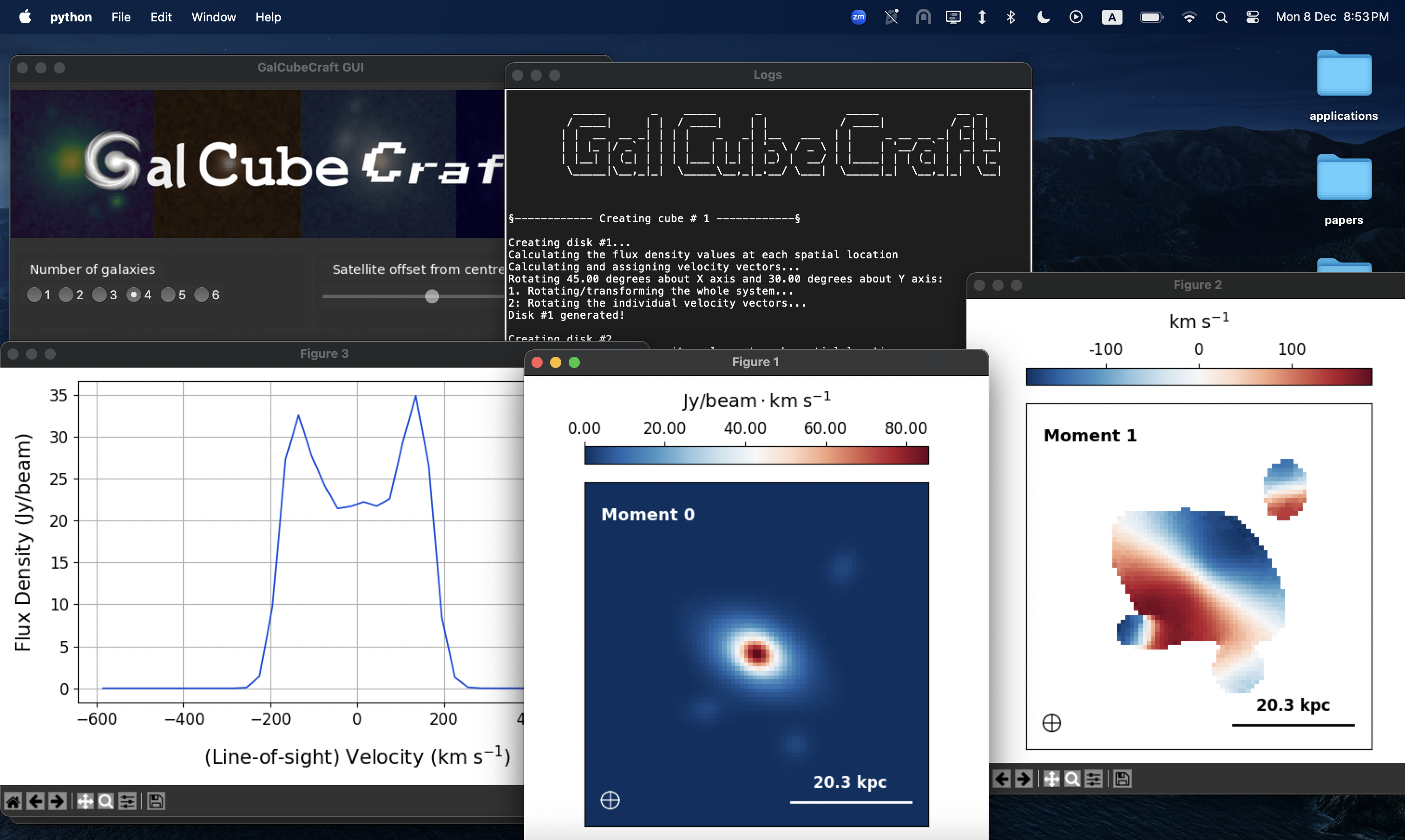
Runs the heavy generation step in a background thread and displays logs in a small Log window so you can follow progress and any printed diagnostics.
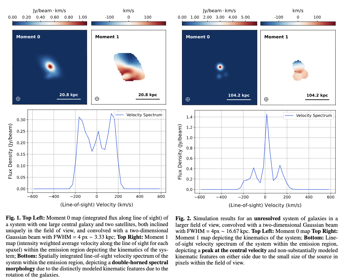
Provides convenience buttons to visualise results using the plotting helpers: Moment-0 (integrated intensity), Moment-1 (intensity-weighted velocity), and the integrated line-of-sight spectrum. These open interactive Matplotlib figures so you can pan/zoom as needed.
Allows saving the generated spectral cube along with a parameters/metadata dictionary to disk. Both NumPy
.npzarchives and Python.pklpickles are supported by the GUI save dialog.
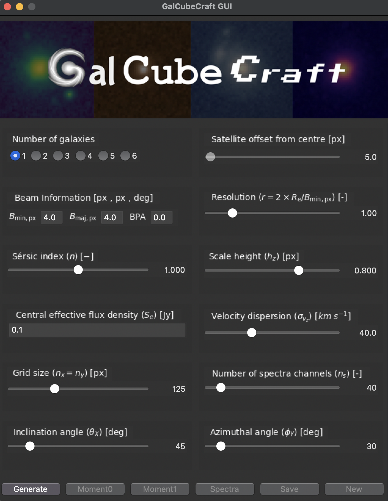
Controls and parameters#
The GUI exposes the following user-adjustable parameters (each control is
directly reflected in the generator instance shown in gui.py):
Number of galaxies (primary + satellites)
Satellite offset (distance from primary centre, pixels)
Beam information: minor axis (bmin, px), major axis (bmaj, px), position angle (BPA, degrees)
Resolution parameter r (controls Re relative to beam size)
Sérsic index n (profile concentration)
Scale height h_z (vertical exponential scale, px)
Central effective flux density S_e (intrinsic scaling)
Line-of-sight velocity dispersion σ_v,z (km/s)
Grid size (nx = ny, pixels)
Number of spectral channels (n_s)
Inclination angle (rotation about X, degrees)
Azimuthal / position angle (rotation about Y, degrees)
Behaviour and UX notes#
Generation is started with the “Generate” button. While a cube is being produced the GUI disables the interactive sliders (to indicate a running state) and the Log window is shown so you can follow output.
When generation finishes the visualisation buttons (Moment0, Moment1, Spectra) and the Save button become enabled. The “New” button clears the current generator state and re-enables controls so you can start a fresh instance.
The GUI attempts to render LaTeX-style labels for parameter names (using Matplotlib mathtext). If rendering fails for a label it falls back to a readable plain-text label so controls remain understandable.
Visualisation#
Moment-0: integrated intensity map produced by summing the cube along the spectral axis and optionally saving the figure.
Moment-1: intensity-weighted velocity map computed from the spectral channels and visualised with an overlaid beam marker.
Spectrum: integrated flux vs velocity (line-of-sight spectrum).
All visualisation helpers are implemented as small functions in
src/GalCubeCraft/visualise.py and are called by the GUI to produce Matplotlib
figures. These figures are interactive; you can pan/zoom and save them using
Matplotlib’s GUI controls.
Saving#
The GUI Save flow prefers to save already-generated results (so it does not re-run the expensive generation step). You can save as a compressed NumPy archive (
.npz) or as a pickled Python object (.pkl). Saved contents include the spectral cube array and a parameter dictionary with metadata (beam info, pixel scale, average velocities, etc.).
Future features#
Planned enhancements for future releases include:
Artificial noise injection and configurable S/N controls
Batch generation of multiple cubes and export of training-ready datasets
More advanced kinematic models and multi-component morphologies
Small GUI refinements (progress bar for generation, better layout on HiDPI displays)
See the src/GalCubeCraft/gui.py source for implementation details and the
complete mapping between UI controls and generator parameters.
Troubleshooting#
Import error after pip install: check that
PYTHONPATHis not shadowing the installed package and that you’re using the same Python interpreter wherepipinstalled the package (usepython -m pip install ...to be explicit).If plotting fails, ensure GUI backend is available or use a non-interactive backend (e.g.,
matplotlib.use('Agg')) when running headless.
Credits & citation#
This package was developed as a compact educational and research tool for IFU data simulation and denoising algorithm development. If you use GalCubeCraft in published work, please cite the following paper:
Lahiry, A., Díaz-Santos, T., Starck, J.-L., Roy, N. C., Anglés-Alcázar, D., Tsagkatakis, G., & Tsakalides, P.
Deep and Sparse Denoising Benchmarks for Spectral Data Cubes of High-z Galaxies: From Simulations to ALMA Observations.
Submitted to Astronomy & Astrophysics (A&A), 2025.
License: MIT — see the LICENSE file in this repository for the full text.